12. Causal Inference

import pandas as pd
from pandas import Series, DataFrame
import numpy as np
import matplotlib.pyplot as plt 
%matplotlib inline
import seaborn as sns
import chardet
import json

import graphviz as gr

import pickle 
import econml   ## install package using cmd 
import dowhy    ## install using cmd 
from dowhy import CausalModel
from IPython.display import Image, display 

import statistics
from scipy.stats import shapiro
import scipy.stats as stats
from scipy.stats import mannwhitneyu, ks_2samp
import warnings
from sklearn.exceptions import ConvergenceWarning
warnings.simplefilter(action='ignore', category=FutureWarning)
warnings.simplefilter("ignore", category=ConvergenceWarning)
from termcolor import colored

from sklearn import datasets
import statsmodels.formula.api as sm
import econtools.metrics as mt

Causal inference is the leveraging of theory and deep knowledge of institutional details to estimate the impact of events and choices on a given outcome of interest. In the field of economics, we find data from experimental studies or observational data. Each of them presents its own challenges to estimate unbiased causal effect.

1. The challenging to identify causal effect: correlation is not causation

Confunding bias: treatment and the outcome shares a common cause

Take the following example, since the beginning of the last century there has been much debate about the cause of the sustained increase in lung cancer. Initial data indicated that there was a statistical association between smoking and lung cancer. But ¿how test that causal hypothesis?. Even more so if some doctors argued that genetic factors affects smoking as well as lung cancer independently.This is presented in the following Directed Acyclic Graphs:

Change in genetic factors alters the probability of smoking and, at the same time, the development of cancer. In this way, the relationship between smoking and developing lung cancer would be a spurious correlation or non-causal correlation.

The genetic factor variable is called a confounder because. Confounder varaible opens a backdoor-path that creates a non-causal correlation between variables. If the confounding variables are not taken into account, the estimated causal effect will be biased due to the omission of variables. Confounder variables can be observable or unobservable as in the example. The case of an observable confounder would be the education of the parents in the relationship between years of education and labor income.

\( Smoking \rightarrow Lung \ \ Cancer\) Directed causal effect

\( Genetic \ \ factors \rightarrow Smoking \rightarrow Lung \ \ Cancer\) Backdoor-path indirected causal effect

g = gr.Digraph()

g.edge("Genetic Factor", "Smoking"),
g.edge("Genetic Factor", "Lung Cancer"),
g.edge("Smoking", "Lung Cancer")
g

Collider bias: treatment and the outcome shares a common effects

Imagine that with the help of some miracle you are finally able to randomize education in order to measure its effect on wage. But just to be sure you won’t have confounding, you control for a lot of variables, one of them investment. But investment is a common effect that it’s called collider. By conditioning on investment, you are opening a second path between the treatment and the outcome, which will make bias causal effect.

\( Education \rightarrow Labor \ \ Income\) Directed causal effect

\( Education \rightarrow Investment \ ; \ Labor \ \ income \rightarrow Investment \) Backdoor-path indirected causal effect

g = gr.Digraph()

g.edge("Educ", "Investments")
g.edge("Educ", "Wage")
g.edge("Wage", "Investments")

g

2. Potencial outcomes \(Y_i^1 \ \ Y_i^0 \)

\(D_i\) is a binary variable that takes on a value of 1 if a particular unit i receives the treatment and a 0 if it does not. Each unit will have two potential outcomes, but only one observed outcome. Potential outcomes are defined as \(Y_i^1\) if unit received the treatment and as \(Y_i^0\) if the unit did not.

A unit’s observable outcome is a function of its potential outcomes determined according to the switching equation

\[ Y_i = Y_i^1 + (1-D_i)*Y_i^0 \]

The unit-specific treatment effect as the difference between the two states of the world:

\[ \delta_i = Y_i^1 - Y_i^0 \]

This requires knowing two states of the world, but we observe only one. Hence, we cannot calculate the unit treatment effect: “counterfactual problem”.

2.1 Average treatment effect

Difference on population expected means in two states of the world.

\[ ATE = E[\delta_i] = E[Y_i^1] - E[Y_i^0] \]

We have to estimate ATE because we just one state if the world. We need to find a valid counterfactual.

How estiamte ATE

\[ ATE = E[Y^1_i | T =1 ] - E[Y^0_i | T =0 ]\]

\[ ATE = ( E[Y^1_i | T =1 ] - E[Y^0_i | T =1 ] ) + E[Y^0_i | T =1 ]- E[Y^0_i | T =0 ] \]

\[ ATE = ATET + E[Y^0_i | T =1 ]- E[Y^0_i | T =0 ] = ATET + (selection \ \ bias) \]

2.1.1 Independece Asumption

\[ (Y^1,Y^0) \ \ | \ \ T \]

Potencial outcome are not correlated to treatment. This eliminates selection bias. In other word, treated and untreated unites are comparable.

2.1.2 SUTVA asumption ( stable unit treatment value assumption)

It implies two things: the treatment is homogeneous between the treated units and there is no spillobes effect. That is, there are no untreated units that receive treatment

2.2 Random Control Trails (RCT)

Randomised Experiments. Randomised experiments consist of randomly assigning individuals in a population to a treatment or to a control group.

Randomisation annihilates bias by making the potential outcomes independent of the treatment. Both groups are comparable into observable and non-observable variables.

\[ ATE = ATET + (selection \ \ bias) = ATET \]

2.3 Internal and external validity:

Random selection keeps características from population (external validity). In a similar way, RCT keeps treatment and control group caracteristics (internal validity). Once treatment, both groups are affected by same external factors. Treatment is the unique difference in both groups. RCT overcome selection bias: accurate estimate of contrafactual.

External validity let to extrapolate or generalized conclusion from sample evaluation to la población de unidades elegibles or targeret popultaion.

3 A/B test

Randomized experimentation process where in two or more versions of a variable (web page, page element, etc.) are shown to different segments of website visitors at the same time to determine which version leaves the maximum impact and drive business metrics.

A/B test application

An ecommerce company used the following strategy: assign discount benefits on online purchases to its customers randomly. The notice of benefits will appear in the user’s virtual account. This strategy is applied for one year.

The objective of the work is to evaluate the causal effect of the marketing strategy. Does the strategy manage to increase sales? Does the marketing strategy increase sales in a sustained manner?

# Uplaoad base from marketing strategies 

base = open(r'../_data/ABtest/abtest.csv', 'rb').read()
det = chardet.detect(base)
charenc = det['encoding']

base1 = pd.read_csv( r'../_data/ABtest/abtest.csv', encoding = charenc)
base1 

	user_id	signup_month	month	spend	treatment
0	0	8	1	511	True
1	0	8	2	471	True
2	0	8	3	465	True
3	0	8	4	479	True
4	0	8	5	429	True
...	...	...	...	...	...
119995	9999	8	8	399	True
119996	9999	8	9	488	True
119997	9999	8	10	524	True
119998	9999	8	11	494	True
119999	9999	8	12	509	True

120000 rows × 5 columns

	user_id	signup_month	month	spend	treatment
0	0	8	1	511	True
1	0	8	2	471	True
2	0	8	3	465	True
3	0	8	4	479	True
4	0	8	5	429	True
...	...	...	...	...	...
119995	9999	8	8	399	True
119996	9999	8	9	488	True
119997	9999	8	10	524	True
119998	9999	8	11	494	True
119999	9999	8	12	509	True

120000 rows × 5 columns

base = base1.replace({True: 1, False: 0})
base.dtypes

user_id         int64
signup_month    int64
month           int64
spend           int64
treatment       int64
dtype: object

user_id         int64
signup_month    int64
month           int64
spend           int64
treatment       int64
dtype: object

# The function and bucle allows to identify the benefits per month and accumulated sales. 

def causal_signup_month(a,i,j):
    data = a[(a.signup_month == i) | (a.signup_month == 0)]
    data = data[(data.month >= i) & (data.month <= i+j)]
    data = data.groupby(['user_id'], as_index=False)['spend','treatment'].sum()
    data['treatment'] =  data['treatment']/(j+1)
    return data


for j in range(1,12):
    for i in range(1,12):
        globals()[f'base_{i}_{j+1}'] = causal_signup_month(base,i,j)

# total sales under two months of treatment for the beneficiary clients on (February)
# sales under treatment (February and march)

base_2_2

	user_id	spend	treatment
0	1	926	0.0
1	2	922	0.0
2	3	1010	1.0
3	4	958	0.0
4	9	945	0.0
...	...	...	...
5458	9990	999	0.0
5459	9992	918	0.0
5460	9995	940	0.0
5461	9996	992	0.0
5462	9998	963	0.0

5463 rows × 3 columns

	user_id	spend	treatment
0	1	926	0.0
1	2	922	0.0
2	3	1010	1.0
3	4	958	0.0
4	9	945	0.0
...	...	...	...
5458	9990	999	0.0
5459	9992	918	0.0
5460	9995	940	0.0
5461	9996	992	0.0
5462	9998	963	0.0

5463 rows × 3 columns

# total sales under three months of treatment for the beneficiary clients on June
# months under treatment (June, July and August)

base_6_3

	user_id	spend	treatment
0	1	1296	0.0
1	2	1296	0.0
2	4	1285	0.0
3	6	1500	1.0
4	9	1311	0.0
...	...	...	...
5472	9993	1589	1.0
5473	9995	1241	0.0
5474	9996	1308	0.0
5475	9997	1504	1.0
5476	9998	1253	0.0

5477 rows × 3 columns

	user_id	spend	treatment
0	1	1296	0.0
1	2	1296	0.0
2	4	1285	0.0
3	6	1500	1.0
4	9	1311	0.0
...	...	...	...
5472	9993	1589	1.0
5473	9995	1241	0.0
5474	9996	1308	0.0
5475	9997	1504	1.0
5476	9998	1253	0.0

5477 rows × 3 columns

# Kolmorogov - Smirnov Test: independent sample from common population distribution f(X)

ks_2samp(base_2_2['spend'][base_2_2.treatment == 1], base_2_2['spend'][base_2_2.treatment == 0])

# H0: samples come from same population distribution
# Pvalues is less than 5%, therefore the null hypothesis that both samples come from the same distribution is rejected.

KstestResult(statistic=0.8733908806150343, pvalue=8.7e-322, statistic_location=997, statistic_sign=-1)

KstestResult(statistic=0.8733908806150343, pvalue=8.7e-322, statistic_location=997, statistic_sign=-1)

test_1 = base_2_2.groupby("treatment")['spend'].agg(["count","mean","std","median","min","max"])
test_1 

# Mean are different in both group

	count	mean	std	median	min	max
treatment
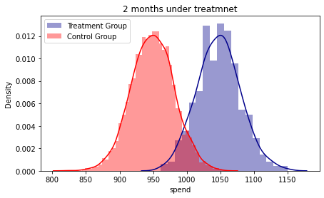
0.0	5006	949.386536	32.057687	949.0	819	1058
1.0	457	1047.463895	32.159405	1047.0	961	1150

	count	mean	std	median	min	max
treatment
0.0	5006	949.386536	32.057687	949.0	819	1058
1.0	457	1047.463895	32.159405	1047.0	961	1150

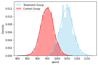
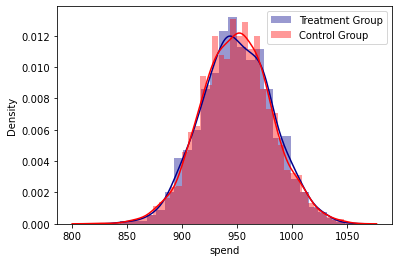
sns.distplot( base_2_2['spend'][base_2_2.treatment == 1] , color="skyblue", label="Treatment Group")
sns.distplot( base_2_2['spend'][base_2_2.treatment == 0] , color="red", label="Control Group")
plt.legend()
plt.show()

# Different densities corroborated the first test

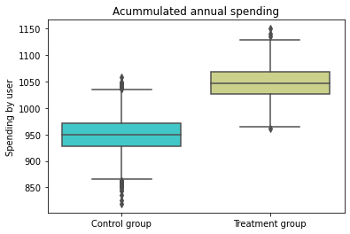
box = sns.boxplot(x="treatment", y="spend", data = base_2_2, palette='rainbow')
plt.ylabel('Spending by user')
plt.xlabel('')
plt.title('Acummulated annual spending')
(box.set_xticklabels(["Control group", "Treatment group"]));

jb1 = stats.jarque_bera(base_2_2["spend"][base_2_2.treatment == 1])
jb2 = stats.jarque_bera(base_2_2["spend"][base_2_2.treatment == 0])
print(jb1)
print(jb2)
# H0: samples come from Normal distribution

# Pvalues is larger than 5%, even 10%,, therefore, the null hypothesis that the
# samples were drawn from a normal distribution is not rejected.

SignificanceResult(statistic=1.0913765748896174, pvalue=0.5794428228359012)
SignificanceResult(statistic=0.9621851872679125, pvalue=0.6181076822166733)

 t_value, t_test_p = stats.ttest_ind(base_2_2["spend"][base_2_2.treatment == 1], 
                                     base_2_2["spend"][base_2_2.treatment == 0], equal_var=False)
    
print('t_value = %.3f, t_test_p = %.3f' % (t_value, t_test_p),"\n")
# H0: samples come from same population distribution
# Non-parametric test that corroborates that both samples come from different distributions because p-vales is less 5%. 

t_value = 62.426, t_test_p = 0.000 

t_value, t_test_p = stats.mannwhitneyu(base_2_2["spend"][base_2_2.treatment == 1], base_2_2["spend"][base_2_2.treatment == 0])
print('statistics-t = %.3f, P_value= %.3f' % (t_value, t_test_p),"\n")

# H0: mean(y)treatment = mean(y)control
#  p-vales is less 5%, hence H0 is rejected. The average sales of both groups is statistically different.

statistics-t = 2254562.000, P_value= 0.000 

mod = sm.ols('spend ~ treatment', data=base_2_2)
res = mod.fit()
print(res.summary())

# For the beneficiaries of the month of February, the first two months undrer treatment increased sales by 98.07 dollars compared to the non-beneficiary group. 
# This result is statistically significant at the 95% confidence level.
# the coefficient does not present important bias since the treatment and control groups are statistically comparable.
# Hence, no bias due to omission of relevant variables

                            OLS Regression Results                            
==============================================================================
Dep. Variable:                  spend   R-squared:                       0.418
Model:                            OLS   Adj. R-squared:                  0.418
Method:                 Least Squares   F-statistic:                     3918.
Date:                Fri, 07 Apr 2023   Prob (F-statistic):               0.00
Time:                        22:25:25   Log-Likelihood:                -26695.
No. Observations:                5463   AIC:                         5.339e+04
Df Residuals:                    5461   BIC:                         5.341e+04
Df Model:                           1                                         
Covariance Type:            nonrobust                                         
==============================================================================
                 coef    std err          t      P>|t|      [0.025      0.975]
------------------------------------------------------------------------------
Intercept    949.3865      0.453   2094.793      0.000     948.498     950.275
treatment     98.0774      1.567     62.591      0.000      95.005     101.149
==============================================================================
Omnibus:                        0.827   Durbin-Watson:                   1.984
Prob(Omnibus):                  0.661   Jarque-Bera (JB):                0.780
Skew:                           0.001   Prob(JB):                        0.677
Kurtosis:                       3.059   Cond. No.                         3.64
==============================================================================

Notes:
[1] Standard Errors assume that the covariance matrix of the errors is correctly specified.

def abtest(base):

    print(colored("Kolmorogov - Smirnov Test","cyan", attrs=["bold"]),"\n")
    t_value, t_test_p = ks_2samp(base['spend'][base.treatment == 1], base['spend'][base.treatment == 0])
    print('t_value = %.3f, t_test_p = %.3f' % (t_value, t_test_p),"\n")
    
    print(colored("Summary Statistics","cyan", attrs=["bold"]),"\n")
    test_1 = base.groupby("treatment")['spend'].agg(["count","mean","std","median","min","max"])
    print(test_1, "\n")
    
    print(colored("Jarque Bera Normality Test","cyan", attrs=["bold"]),"\n")
    jb1 = stats.jarque_bera(base["spend"][base.treatment == 1])
    jb2 = stats.jarque_bera(base["spend"][base.treatment == 0])
    print(f'Jarque Bera (treatment group): {jb1}', "\n")
    print(f'Jarque Bera (control group):  {jb2}', "\n")

    print(colored("Mann Whitney U Non parametric - Test","cyan", attrs=["bold"]),"\n")
    t_value, t_test_p = stats.mannwhitneyu(base["spend"][base.treatment == 1], base["spend"][base.treatment == 0])
    print('statistics-t = %.3f, P_value= %.3f' % (t_value, t_test_p),"\n")

    print(colored("T-test mean","cyan", attrs=["bold"]),"\n")
    t_value, t_test_p = stats.ttest_ind(base["spend"][base.treatment == 1], 
                                     base["spend"][base.treatment == 0], equal_var=False)
    print('t_value = %.3f, t_test_p = %.3f' % (t_value, t_test_p),"\n")
    
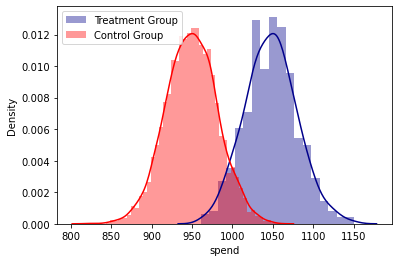
    print(colored("Densities Plot analysis", "cyan", attrs=["bold"]),"\n")
    sns.distplot( base['spend'][base.treatment == 1] , color="darkblue", label="Treatment Group")
    sns.distplot( base['spend'][base.treatment == 0] , color="red", label="Control Group")
    plt.legend()
    plt.show()

    print(colored("Regression analysis", "cyan", attrs=["bold"]),"\n")
    mod = sm.ols('spend ~ treatment', data=base)
    res = mod.fit()
    print(res.summary(),"\n")
    
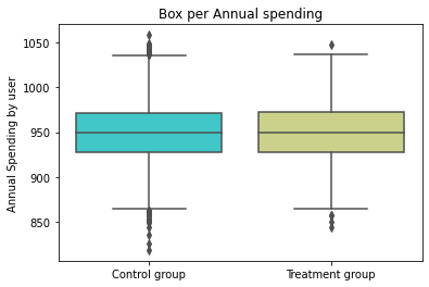
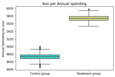
    print(colored("Pox Plot analysis", "cyan", attrs=["bold"]),"\n")
    box = sns.boxplot(x="treatment", y="spend", data= base, palette='rainbow')
    plt.ylabel('Annual Spending by user')
    plt.xlabel('')
    plt.title('Box per Annual spending')
    (box.set_xticklabels(["Control group", "Treatment group"]))

abtest(base_2_2)

Kolmorogov - Smirnov Test 

t_value = 0.873, t_test_p = 0.000 

Summary Statistics 

           count         mean        std  median  min   max
treatment                                                  
0.0         5006   949.386536  32.057687   949.0  819  1058
1.0          457  1047.463895  32.159405  1047.0  961  1150 

Jarque Bera Normality Test 

Jarque Bera (treatment group): SignificanceResult(statistic=1.0913765748896174, pvalue=0.5794428228359012) 

Jarque Bera (control group):  SignificanceResult(statistic=0.9621851872679125, pvalue=0.6181076822166733) 

Mann Whitney U Non parametric - Test 

statistics-t = 2254562.000, P_value= 0.000 

T-test mean 

t_value = 62.426, t_test_p = 0.000 

Densities Plot analysis 

Regression analysis 

                            OLS Regression Results                            
==============================================================================
Dep. Variable:                  spend   R-squared:                       0.418
Model:                            OLS   Adj. R-squared:                  0.418
Method:                 Least Squares   F-statistic:                     3918.
Date:                Fri, 07 Apr 2023   Prob (F-statistic):               0.00
Time:                        22:25:30   Log-Likelihood:                -26695.
No. Observations:                5463   AIC:                         5.339e+04
Df Residuals:                    5461   BIC:                         5.341e+04
Df Model:                           1                                         
Covariance Type:            nonrobust                                         
==============================================================================
                 coef    std err          t      P>|t|      [0.025      0.975]
------------------------------------------------------------------------------
Intercept    949.3865      0.453   2094.793      0.000     948.498     950.275
treatment     98.0774      1.567     62.591      0.000      95.005     101.149
==============================================================================
Omnibus:                        0.827   Durbin-Watson:                   1.984
Prob(Omnibus):                  0.661   Jarque-Bera (JB):                0.780
Skew:                           0.001   Prob(JB):                        0.677
Kurtosis:                       3.059   Cond. No.                         3.64
==============================================================================

Notes:
[1] Standard Errors assume that the covariance matrix of the errors is correctly specified. 

Pox Plot analysis 

#Positive causal effect of the marketing strategy over time

coef = pd.DataFrame(columns=('months','causal_effect', 'lower','upper'))
                    
for j in range(2,12):
    mod = sm.ols('spend ~ treatment', data=globals()[f'base_2_{j}'])
    res = mod.fit()
    coef.loc[j-2,'lower']=res.conf_int(alpha=0.05, cols=None)[0][1]
    coef.loc[j-2,'upper']=res.conf_int(alpha=0.05, cols=None)[1][1]
    coef.loc[j-2,'causal_effect']=res.params[1]
    coef.loc[j-2,'months']= j

coef

	months	causal_effect	lower	upper
0	2	98.077359	95.005482	101.149236
1	3	198.97023	195.249432	202.691028
2	4	299.287842	295.014514	303.56117
3	5	400.08003	395.333792	404.826269
4	6	500.627491	495.414822	505.840161
5	7	602.782273	597.151287	608.413259
6	8	703.938904	697.942304	709.935505
7	9	805.135222	798.744774	811.525669
8	10	1005.810219	998.792173	1012.828265
9	11	1005.810219	998.792173	1012.828265

    fig, axes = plt.subplots(figsize=(7, 4))                             
    ax1 = sns.distplot( base_2_2['spend'][base_2_2.treatment == 1] , color="darkblue", label="Treatment Group")
    ax1 = sns.distplot( base_2_2['spend'][base_2_2.treatment == 0] , color="red", label="Control Group")
    plt.title('2 months under treatmnet')
    plt.legend()
    
    fig, ax = plt.subplots(figsize=(7, 4))  
    ax2 = sns.distplot( base_2_6['spend'][base_2_6.treatment == 1] , color="darkblue", label="Treatment Group")
    ax2 = sns.distplot( base_2_6['spend'][base_2_6.treatment == 0] , color="red", label="Control Group")
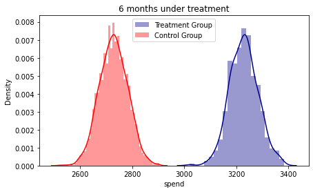
    plt.title('6 months under treatment')
    plt.legend()
    
    fig, ax = plt.subplots(figsize=(7, 4))  
    ax3 = sns.distplot( base_2_10['spend'][base_2_10.treatment == 1] , color="darkblue", label="Treatment Group")
    ax3 = sns.distplot( base_2_10['spend'][base_2_10.treatment == 0] , color="red", label="Control Group")
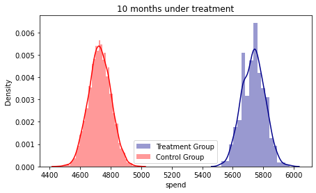
    plt.title('10 months under treatment')
    plt.legend()
    
    #The densities show an increasing gap according to the months accumulated under the treatment.
    #Treatment clients on february

<matplotlib.legend.Legend at 0x1f0445ac8e0>

base_2_10 = causal_signup_month(base,2,10)

# AB test for ten months under treatment for the beneficiary clients on February
abtest(base_2_10)

Kolmorogov - Smirnov Test 

t_value = 1.000, t_test_p = 0.000 

Summary Statistics 

           count         mean        std  median   min   max
treatment                                                   
0.0         5006  4728.382341  73.222369  4728.0  4456  4988
1.0          457  5734.192560  73.657384  5737.0  5525  5970 

Jarque Bera Normality Test 

Jarque Bera (treatment group): SignificanceResult(statistic=0.4653152162176708, pvalue=0.7924248469227017) 

Jarque Bera (control group):  SignificanceResult(statistic=0.6594857909581255, pvalue=0.7191085957374495) 

Mann Whitney U Non parametric - Test 

statistics-t = 2287742.000, P_value= 0.000 

T-test mean 

t_value = 279.577, t_test_p = 0.000 

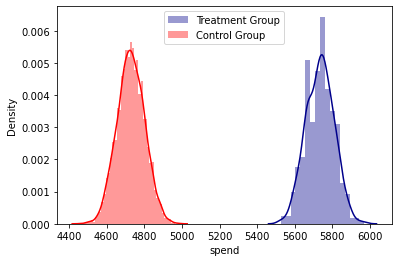
Densities Plot analysis 

Regression analysis 

                            OLS Regression Results                            
==============================================================================
Dep. Variable:                  spend   R-squared:                       0.935
Model:                            OLS   Adj. R-squared:                  0.935
Method:                 Least Squares   F-statistic:                 7.894e+04
Date:                Fri, 07 Apr 2023   Prob (F-statistic):               0.00
Time:                        22:25:53   Log-Likelihood:                -31209.
No. Observations:                5463   AIC:                         6.242e+04
Df Residuals:                    5461   BIC:                         6.243e+04
Df Model:                           1                                         
Covariance Type:            nonrobust                                         
==============================================================================
                 coef    std err          t      P>|t|      [0.025      0.975]
------------------------------------------------------------------------------
Intercept   4728.3823      1.035   4566.656      0.000    4726.353    4730.412
treatment   1005.8102      3.580    280.960      0.000     998.792    1012.828
==============================================================================
Omnibus:                        0.918   Durbin-Watson:                   2.000
Prob(Omnibus):                  0.632   Jarque-Bera (JB):                0.947
Skew:                           0.003   Prob(JB):                        0.623
Kurtosis:                       2.936   Cond. No.                         3.64
==============================================================================

Notes:
[1] Standard Errors assume that the covariance matrix of the errors is correctly specified. 

Pox Plot analysis 

#Placebo Test: Treatment groups are artificially created from control group. 
# Beneficiary units are randomly selected from the control group

# artificial beneficiary clients of february
j = 2

pbo_base0 = base[base.treatment == 0].drop('treatment', axis =1)
pbo_base1 = pbo_base0.drop_duplicates(subset=['user_id'])

pbo_base1 = pbo_base1.sample(frac=0.25, replace=False, random_state=100)
pbo_base1 = pbo_base1[['user_id']]
pbo_base1['treatment'] = 1

placebo_base =  pd.merge(pbo_base0, pbo_base1, how="left", on=["user_id"])
placebo_base['treatment'] = placebo_base['treatment'].fillna(0)
placebo_base.loc[placebo_base.treatment == 1, 'signup_month'] = j
globals()[f'placebo_base_{j}'] = placebo_base


# first two months under treatment for february artifical benficiaries
placebo_2_2 = causal_signup_month(placebo_base_2,2,1)

placebo_base_2.describe()

	user_id	signup_month	month	spend	treatment
count	60072.000000	60072.000000	60072.000000	60072.000000	60072.000000
mean	4972.272473	0.500200	6.500000	434.853443	0.250100
std	2890.220110	0.866148	3.452081	41.062485	0.433074
min	1.000000	0.000000	1.000000	286.000000	0.000000
25%	2448.000000	0.000000	3.750000	404.000000	0.000000
50%	5010.000000	0.000000	6.500000	435.000000	0.000000
75%	7475.000000	2.000000	9.250000	466.000000	1.000000
max	9998.000000	2.000000	12.000000	566.000000	1.000000

#Placebo test for artificial beneficiary group on february

abtest(placebo_2_2)

#It can be seen that both groups are statistically equal. 
# There is no evidence that the artificial treatment group has increased their purchases.

Kolmorogov - Smirnov Test 

t_value = 0.019, t_test_p = 0.867 

Summary Statistics 

           count        mean        std  median  min   max
treatment                                                 
0.0         3754  949.257326  32.146578   949.5  819  1058
1.0         1252  949.773962  31.799294   949.0  844  1048 

Jarque Bera Normality Test 

Jarque Bera (treatment group): SignificanceResult(statistic=0.8424322407805283, pvalue=0.6562482574525269) 

Jarque Bera (control group):  SignificanceResult(statistic=2.533146164438528, pvalue=0.2817956595520864) 

Mann Whitney U Non parametric - Test 

statistics-t = 2371435.000, P_value= 0.628 

T-test mean 

t_value = 0.496, t_test_p = 0.620 

Densities Plot analysis 

Regression analysis 

                            OLS Regression Results                            
==============================================================================
Dep. Variable:                  spend   R-squared:                       0.000
Model:                            OLS   Adj. R-squared:                 -0.000
Method:                 Least Squares   F-statistic:                    0.2438
Date:                Fri, 07 Apr 2023   Prob (F-statistic):              0.621
Time:                        22:26:01   Log-Likelihood:                -24461.
No. Observations:                5006   AIC:                         4.893e+04
Df Residuals:                    5004   BIC:                         4.894e+04
Df Model:                           1                                         
Covariance Type:            nonrobust                                         
==============================================================================
                 coef    std err          t      P>|t|      [0.025      0.975]
------------------------------------------------------------------------------
Intercept    949.2573      0.523   1814.120      0.000     948.232     950.283
treatment      0.5166      1.046      0.494      0.621      -1.535       2.568
==============================================================================
Omnibus:                        1.004   Durbin-Watson:                   1.996
Prob(Omnibus):                  0.605   Jarque-Bera (JB):                0.957
Skew:                          -0.010   Prob(JB):                        0.620
Kurtosis:                       3.065   Cond. No.                         2.48
==============================================================================

Notes:
[1] Standard Errors assume that the covariance matrix of the errors is correctly specified. 

Pox Plot analysis 

References

Causal inference

https://towardsdatascience.com/causal-inference-962ae97cefda

https://towardsdatascience.com/a-practical-guide-to-a-b-tests-in-python-66666f5c3b02

https://mixtape.scunning.com/introduction.html

https://theeffectbook.net/introduction.html

A/B test

https://www.kaggle.com/babyoda/a-b-testing-in-practice

https://towardsdatascience.com/ab-testing-with-python-e5964dd66143

https://www.kaggle.com/ekrembayar/a-b-testing-step-by-step-hypothesis-testing